Problem set 5

Due by 11:59 PM on Monday, May 5, 2025

Instructions

Please use an RMarkdown file to complete this assignment. Make sure you reserve code chunks for code and write out any interpretations or explainations outside of code chunks. Submit the knitted PDF file containing your code and written answers on Canvas.

Questions

The data contained in library(MASS);data(eagles) are records of salmon pirating attempts by Bald Eagles in Washington State. See ?eagles for details. While one eagle feeds, sometimes another will swoop in and try to steal the salmon from it. Call the feeding eagle the “victim” and the thief the “pirate.” Use the available data to build a binomial GLM of successful pirating attempts.

Consider the following model:

$\begin{aligned} y_{i} & \sim Binomial (n_{i}, p_{i}) \\ logit (p_{i}) & = α + β_{P} P_{i} + β_{V} V_{i} + β_{A} A_{i} \\ α & \sim Normal (0, 1.5) \\ β_{P}, β_{V}, β_{A} & \sim Normal (0, 0.5) \end{aligned}$

where $y$ is the number of successful attempts, $n$ is the total number of attempts, $P$ is a dummy variable indicating whether or not the pirate had large body size, $V$ is a dummy variable indicating whether or not the victim had large body size, and finally $A$ is a dummy variable indicating whether or not the pirate was an adult. Fit the model above to the eagles data.

Click to see the answer

# Load required libraries
library(brms)

Loading required package: Rcpp

Loading 'brms' package (version 2.22.0). Useful instructions
can be found by typing help('brms'). A more detailed introduction
to the package is available through vignette('brms_overview').


Attaching package: 'brms'

The following object is masked from 'package:stats':

    ar

library(tidyverse)

── Attaching core tidyverse packages ──────────────────────── tidyverse 2.0.0 ──
✔ dplyr     1.1.4     ✔ readr     2.1.5
✔ forcats   1.0.0     ✔ stringr   1.5.1
✔ ggplot2   3.5.1     ✔ tibble    3.2.1
✔ lubridate 1.9.3     ✔ tidyr     1.3.1
✔ purrr     1.0.2

── Conflicts ────────────────────────────────────────── tidyverse_conflicts() ──
✖ dplyr::filter() masks stats::filter()
✖ dplyr::lag()    masks stats::lag()
ℹ Use the conflicted package (<http://conflicted.r-lib.org/>) to force all conflicts to become errors

library(tidybayes)


Attaching package: 'tidybayes'

The following objects are masked from 'package:brms':

    dstudent_t, pstudent_t, qstudent_t, rstudent_t

library(patchwork)
library(here)

here() starts at /Users/sweston2/Library/CloudStorage/GoogleDrive-weston.sara@gmail.com/My Drive/Work (google drive)/teaching/uobayes

library(cowplot)


Attaching package: 'cowplot'

The following object is masked from 'package:patchwork':

    align_plots

The following object is masked from 'package:lubridate':

    stamp

theme_set(theme_cowplot())

# Load and examine the data
data(eagles, package = "MASS")
d <- eagles
rethinking::precis(d)

  mean        sd  5.5%  94.5%     histogram
y 12.5 10.663690 0.385 25.535        ▇▁▂▇▁▂
n 20.0  8.831761 7.080 28.615 ▃▁▁▃▁▃▁▃▁▃▁▇▃
P  NaN        NA    NA     NA              
A  NaN        NA    NA     NA              
V  NaN        NA    NA     NA

d %>% count(P, V, A)

  P V A n
1 L L A 1
2 L L I 1
3 L S A 1
4 L S I 1
5 S L A 1
6 S L I 1
7 S S A 1
8 S S I 1

# Fit the model using brms
m1 <- brm(
  data = d,
  family = binomial,
  y | trials(n) ~ P + V + A,
  prior = c(
    prior(normal(0, 1.5), class = Intercept),
    prior(normal(0, 0.5), class = b)
  ),
  iter = 2000, warmup = 1000, chains = 4, cores = 4,
  seed = 11,
  file = here("files/models/hw5.1")
)

# Display model summary
summary(m1)

 Family: binomial 
  Links: mu = logit 
Formula: y | trials(n) ~ P + V + A 
   Data: eagles (Number of observations: 8) 
  Draws: 4 chains, each with iter = 2000; warmup = 1000; thin = 1;
         total post-warmup draws = 4000

Regression Coefficients:
          Estimate Est.Error l-95% CI u-95% CI Rhat Bulk_ESS Tail_ESS
Intercept     0.90      0.31     0.31     1.53 1.00     4342     3112
PS           -1.64      0.31    -2.24    -1.04 1.00     3734     2888
VS            1.70      0.32     1.09     2.35 1.00     4071     3253
AI           -0.65      0.32    -1.27    -0.04 1.00     3746     3038

Draws were sampled using sampling(NUTS). For each parameter, Bulk_ESS
and Tail_ESS are effective sample size measures, and Rhat is the potential
scale reduction factor on split chains (at convergence, Rhat = 1).

Interpret the estimates and plot the posterior distributions. Compute and display both (1) the predicted probability of success and its 89% interval for each row ( $i$ ) in the data, as well as (2) the predicted success count and its 89% interval. What different information does each type of posterior prediction provide?

Click to see the answer

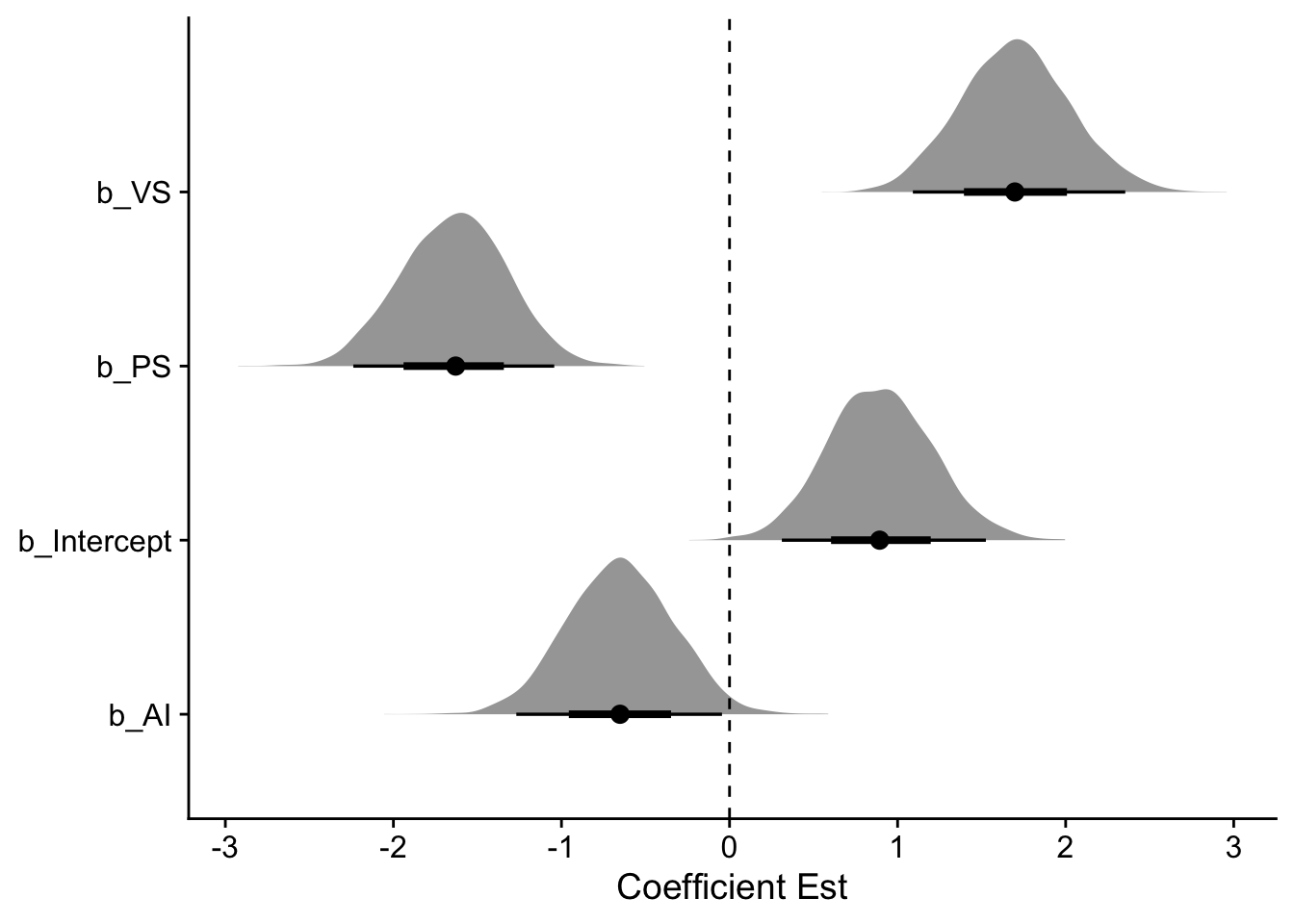
Here’ are the summaries and plots of the coefficient estimates.

# Plot posterior distributions of coefficients
m1 %>% 
  gather_draws(`b_.*`, regex = T) %>% # this will get any variable that starts with b_
  median_qi(.width = .89)

# A tibble: 4 × 7
  .variable   .value .lower .upper .width .point .interval
  <chr>        <dbl>  <dbl>  <dbl>  <dbl> <chr>  <chr>    
1 b_AI        -0.652 -1.15  -0.152   0.89 median qi       
2 b_Intercept  0.893  0.408  1.41    0.89 median qi       
3 b_PS        -1.63  -2.14  -1.15    0.89 median qi       
4 b_VS         1.70   1.19   2.23    0.89 median qi

m1 %>% 
  gather_draws(`b_.*`, regex = T) %>% 
  ggplot( aes( x=.value, y=.variable ) ) +
  stat_halfeye() +
  geom_vline(aes(xintercept=0), linetype="dashed") + 
  labs(x = "Coefficient Est", y=NULL)

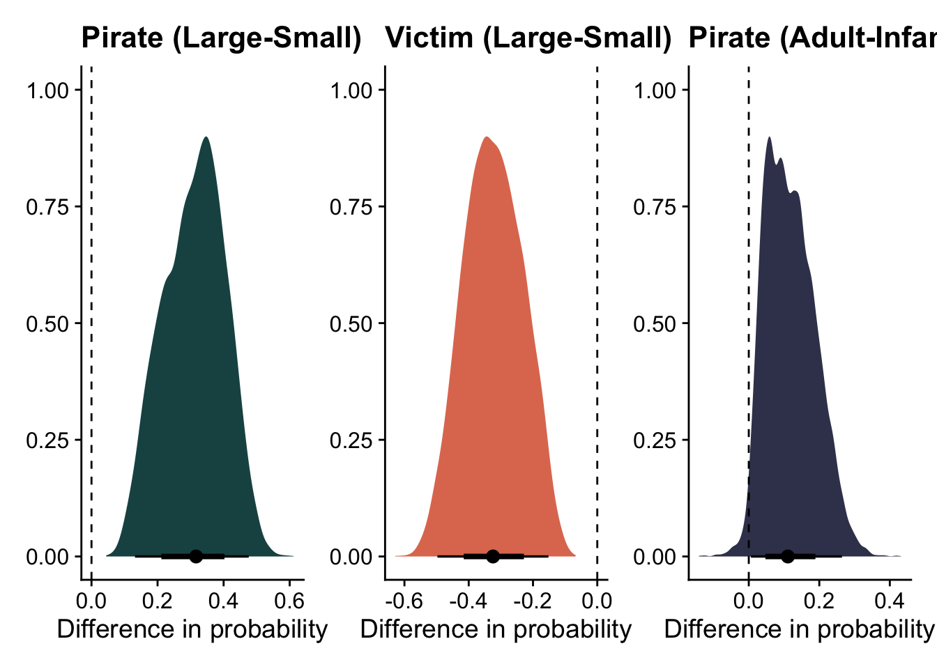
But as we know, in a GLM, these are difficult to interpret. So let’s translate these into probabilites. First, let’s ask how the different coefficients change our probabilities of success.

nd = distinct(eagles, V, P, A) %>% 
  mutate(n = 1e5)
# expected probs
post_epred = nd %>% 
  add_epred_draws(m1) %>% 
  ungroup() %>% 
  mutate(prob = .epred/n) %>% 
  dplyr::select(V, P, A, .draw, prob) 

p1 = post_epred%>% 
  pivot_wider(names_from = P, values_from = prob) %>% 
  mutate(diff = L-S) %>% 
  ggplot(aes( x=diff )) +
  stat_halfeye( fill = "#1c5253") +
  geom_vline(aes(xintercept = 0), linetype ="dashed") +
  labs(x = "Difference in probability", y = NULL, title = "Pirate (Large-Small)")

p2 = post_epred%>% 
  pivot_wider(names_from = V, values_from = prob) %>% 
  mutate(diff = L-S) %>% 
  ggplot(aes( x=diff )) +
  stat_halfeye( fill = "#e07a5f") +
  geom_vline(aes(xintercept = 0), linetype ="dashed") +
  labs(x = "Difference in probability", y = NULL, title = "Victim (Large-Small)")

p3 = post_epred%>% 
  pivot_wider(names_from = A, values_from = prob) %>% 
  mutate(diff = A-I) %>% 
  ggplot(aes( x=diff )) +
  stat_halfeye( fill = "#3d405b") +
  geom_vline(aes(xintercept = 0), linetype ="dashed") +
  labs(x = "Difference in probability", y = NULL, title = "Pirate (Adult-Infant)")

p1 + p2 + p3

Great, these make more sense! Large pirates more successfully steal salmon; smaller victims are more likely to be stolen from; and adult pirates are more successful than infant ones.

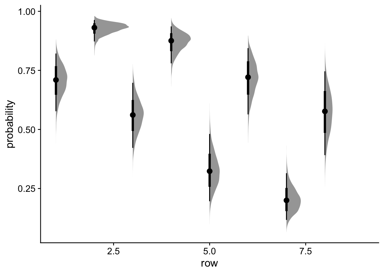
Let’s get the probabilities and counts for each bird in our sample.

epred_draws(m1, newdata = d) %>% 
  ungroup() %>% 
  mutate(prob = .epred/n) %>% 
  ggplot(aes( y=prob, x=.row)) +
  stat_halfeye() +
  labs(x = "row", y = "probability")

epred_draws(m1, newdata = d) %>% 
  ungroup() %>% 
  ggplot(aes( y=.epred, x=.row)) +
  stat_halfeye() +
  labs(x = "row", y = "counts")

The posterior predictions provide two different types of information:

Predicted probabilities :
- Shows the estimated probability of success for each combination of predictors
- Useful for understanding the relative impact of each predictor
- Ranges from 0 to 1
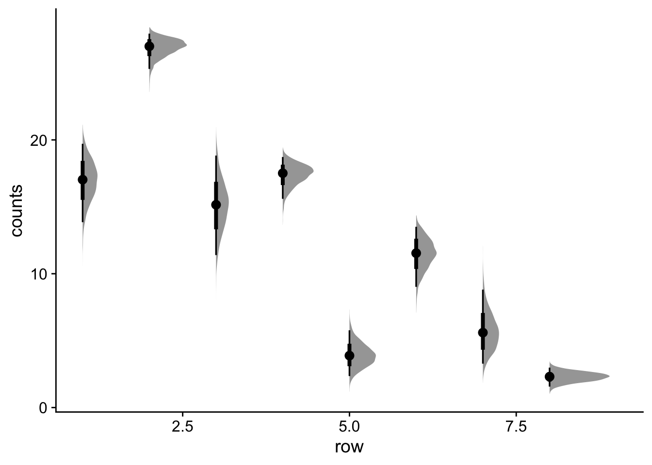
Predicted counts (post_counts):
- Shows the expected number of successful attempts
- Takes into account both the probability and the number of trials
- More directly interpretable in terms of actual outcomes

The key difference is that probabilities show the underlying success rate, while counts show the expected number of successes given the number of attempts. The count predictions are more variable because they incorporate both the uncertainty in the probability and the randomness of the binomial process.

Now try to improve the model. Consider an interaction between the pirate’s size and age (immature or adult). Compare this model to the previous one, using WAIC. Interpret.

Click to see the answer

# Fit the interaction model
m2 <- brm(
  data = d,
  family = binomial,
  y | trials(n) ~ P + V + A + P:A,
  prior = c(
    prior(normal(0, 1.5), class = Intercept),
    prior(normal(0, 0.5), class = b)
  ),
  iter = 2000, warmup = 1000, chains = 4, cores = 4,
  seed = 11,
  file = here("files/models/hw5.2")
)

# Compare models using WAIC
waic(m1, m2) %>% print(simplify=F)

Warning: 
6 (75.0%) p_waic estimates greater than 0.4. We recommend trying loo instead.

Warning: 
5 (62.5%) p_waic estimates greater than 0.4. We recommend trying loo instead.

Output of model 'm1':

Computed from 4000 by 8 log-likelihood matrix.

          Estimate   SE
elpd_waic    -29.5  6.2
p_waic         8.4  3.0
waic          59.1 12.3

6 (75.0%) p_waic estimates greater than 0.4. We recommend trying loo instead. 

Output of model 'm2':

Computed from 4000 by 8 log-likelihood matrix.

          Estimate  SE
elpd_waic    -25.5 4.1
p_waic         7.1 2.3
waic          51.1 8.3

5 (62.5%) p_waic estimates greater than 0.4. We recommend trying loo instead. 

Model comparisons:
   elpd_diff se_diff elpd_waic se_elpd_waic p_waic se_p_waic waic  se_waic
m2   0.0       0.0   -25.5       4.1          7.1    2.3      51.1   8.3  
m1  -4.0       3.7   -29.5       6.2          8.4    3.0      59.1  12.3

# Display model summary
summary(m2)

 Family: binomial 
  Links: mu = logit 
Formula: y | trials(n) ~ P + V + A + P:A 
   Data: d (Number of observations: 8) 
  Draws: 4 chains, each with iter = 2000; warmup = 1000; thin = 1;
         total post-warmup draws = 4000

Regression Coefficients:
          Estimate Est.Error l-95% CI u-95% CI Rhat Bulk_ESS Tail_ESS
Intercept     0.85      0.31     0.24     1.45 1.00     5145     3487
PS           -1.31      0.33    -1.95    -0.67 1.00     4704     3575
VS            1.65      0.33     1.02     2.32 1.00     4301     2981
AI           -0.40      0.33    -1.04     0.24 1.00     4663     3161
PS:AI        -1.11      0.40    -1.89    -0.33 1.00     4404     3423

Draws were sampled using sampling(NUTS). For each parameter, Bulk_ESS
and Tail_ESS are effective sample size measures, and Rhat is the potential
scale reduction factor on split chains (at convergence, Rhat = 1).

The interaction model adds a term P:A to capture how the effect of pirate size (P) varies with age (A). This allows us to test whether the advantage of being a large pirate differs between adult and immature eagles.

The WAIC comparison helps us determine if the more complex model (with interaction) is justified by the data. A lower WAIC indicates better predictive performance, but we should also consider: 1. The magnitude of the WAIC difference 2. The standard error of the difference 3. The complexity of the model

In this case, we improve our prediction a marginal amount – (difference of 4.0 with a standard error of 3.7). In fact, we even have a less complex model (our p_waic is lower for model 2). This can happen when your added parameters capture an important pattern in the data.

Let’s see what we’ve learned from this model.

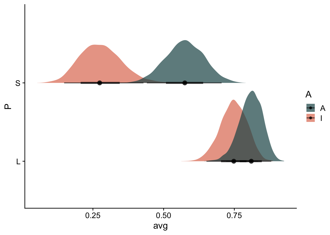
nd = distinct(eagles, V, P, A) %>% 
  mutate(n = 1e5)
# expected probs
nd %>% 
  add_epred_draws(m2) %>% 
  ungroup() %>% 
  mutate(prob = .epred/n) %>% 
  dplyr::select(V, P, A, .draw, prob) %>% 
  pivot_wider(names_from = "V", 
              names_prefix = "V", 
              values_from = prob) %>% 
  mutate(avg = (VL+VS)/2) %>% 
  ggplot(aes( x = avg, y = P, fill = A)) +
  stat_halfeye(alpha=.7) +
  scale_fill_manual(values = c("#1c5253" , "#e07a5f"))

When pirates are large, they are successful regardless of whether they are adults or infants. However, when pirates are small, they are moderately successulf when they are adults, but much less successful when they are infants.