Problem set 2

Due by 11:59 PM on Monday, April 14, 2025

Instructions

Please use an RMarkdown file to complete this assignment. Make sure you reserve code chunks for code and write out any interpretations or explanations outside of code chunks. Submit the knitted PDF file containing your code and written answers on Canvas.

Questions

From the Howell1 dataset, consider only people younger than 13 years old. Estimate the causal association between age and weight. Assume that age influences weight through two paths. First, age influences height, and height influences weight. Second, age directly influences weight through age-related changes in muscle growth and body proportions.

1. Write a generative simulation that takes age as an input and simulates height and weight.

Click to see the answer

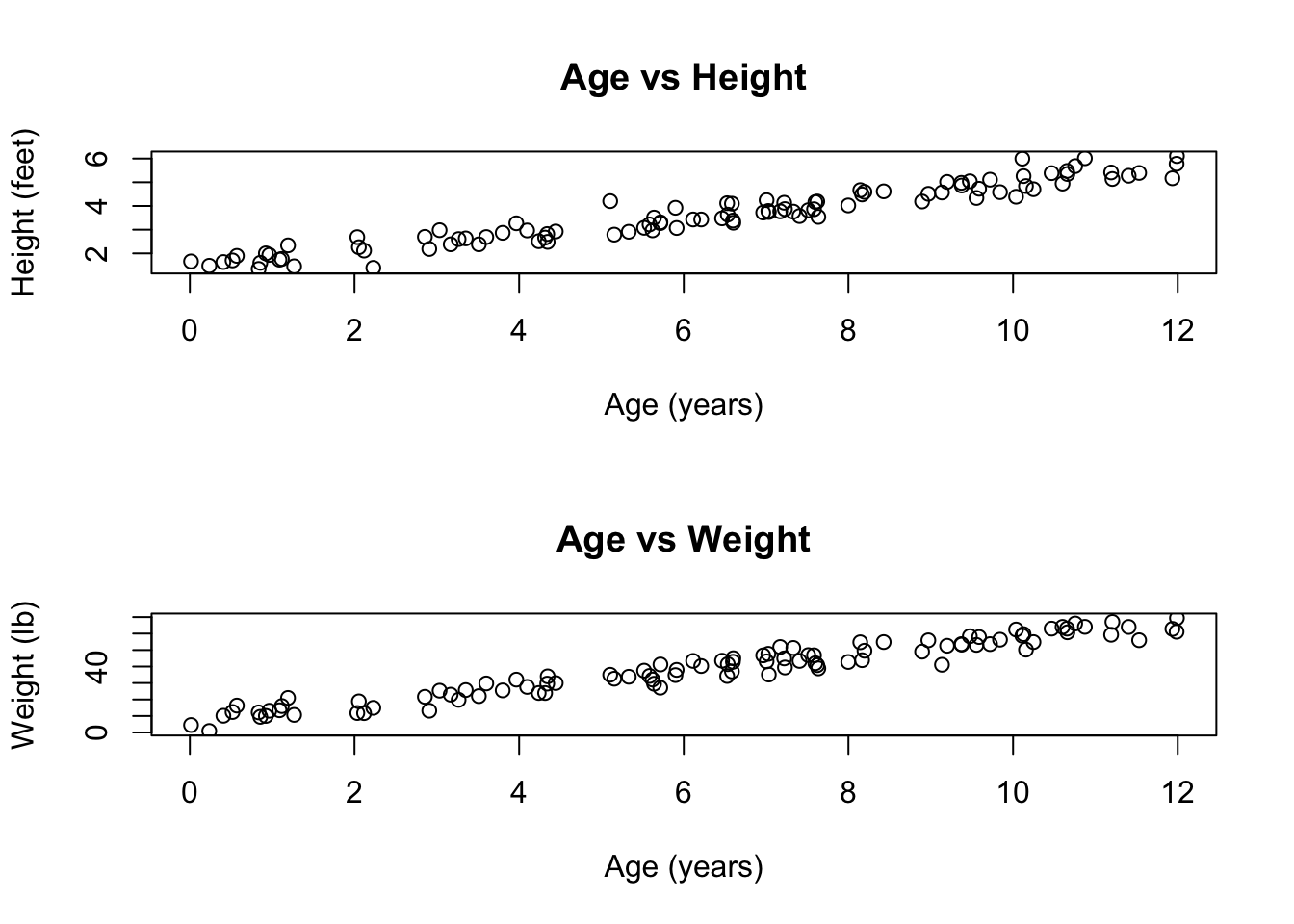
# Define the simulation function
simulate_growth <- function(age) {
  n = length(age)
  # Simulate height (in feet)
  height <- rnorm(n, 
                 mean = 1.5 + .3*age + 0.005*age^2,  # Quadratic growth pattern
                 sd = .3)                           # Random variation
  
  # Simulate weight (in lb)
  weight <- rnorm(n,
                 mean = 6.5 + 5*age + 0.25*height, # Linear relationship with age and height
                 sd = 4)                           # Random variation
  
  data.frame(age=age, height=height, weight=weight)
}

# Generate data for ages 0-12
ages <- runif(100, 0, 12)
sim_data = simulate_growth(ages)

# Plot the simulated relationships
par(mfrow=c(2,1))
plot(sim_data$age, sim_data$height, 
     xlab="Age (years)", ylab="Height (feet)",
     main="Age vs Height")
plot(sim_data$age, sim_data$weight,
     xlab="Age (years)", ylab="Weight (lb)",
     main="Age vs Weight")

This simulation:

1. Takes age as input and generates both height and weight
2. Uses a quadratic function for height to capture the non-linear growth pattern
3. Uses a linear function for weight that depends on both age and height
4. Includes random variation (noise) in both height and weight
5. The plots show the expected relationships: both height and weight increase with age

2. Write out a mathematical model to estimate the linear relationship between age and weight. (Just age, not height!)

Click to see the answer

There are many priors that could be appropriate here. Don’t worry if yours looks different from mine. Here’s just one example:

$$\begin{array}{rl}{W}_i& \sim \text{Normal}({\mu }_i,\sigma )\\ {\mu }_i& =\alpha +({\beta }_A\ast A_i)\\ \alpha & \sim \text{Normal}(7,1.5)\\ {\beta }_A& \sim \text{Normal}(0,1)\\ \sigma & \sim \text{Exponential}(1)\end{array}$$

Where:

• $W_i$ is the weight of individual $i$
• $A_i$ is the age of individual $i$
• $\alpha$ is the intercept
• ${\beta }_A$ is the effect of age on weight
• $\sigma$ is the standard deviation of the weight distribution

This model:

1. Assumes weight is normally distributed around a mean $\mu$
2. The mean $\mu$ is a linear function of age
3. Uses weakly informative priors for all parameters
4. The exponential prior on $\sigma$ ensures it’s positive

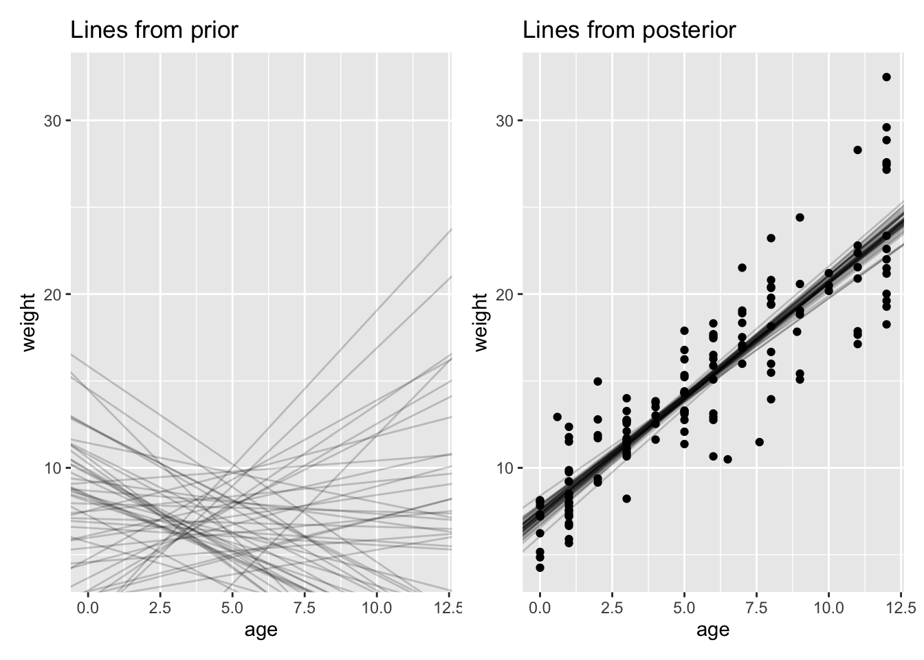
3. Fit this model using brms. Create two plots: one of regression lines implied by your prior and one of the regression lines implied by the posterior.

Click to see the answer

# Load required packages
library(brms)
library(tidyverse)
library(cowplot)
library(patchwork)
data("Howell1", package="rethinking")

# Filter for children under 13
d <- Howell1[Howell1$age < 13,]

# Define the model
mp <- brm(
  weight ~ age,
  data = d,
  prior = c(
    prior(normal(7, 1.5), class = Intercept),
    prior(normal(0, 1), class = b),
    prior(exponential(1), class = sigma)
  ),
  sample_prior = "only"  # First get prior samples
)

# Get prior samples
prior_samples <- as_draws_df(mp)


# Now fit the model with the data
m <- brm(
  weight ~ age,
  data = d,
  prior = c(
    prior(normal(7, 1.5), class = Intercept),
    prior(normal(0, 1), class = b),
    prior(exponential(1), class = sigma)
  )
)

# Get posterior samples
post_samples <- as_draws_df(m)

p1 <- ggplot(d, aes(x=age, y=weight)) + 
  geom_blank() +
  geom_abline(aes(intercept=b_Intercept, slope=b_age),
              data=prior_samples[1:50, ],
              alpha=.2) +
  labs(title="Lines from prior")
p2 <- ggplot(d, aes(x=age, y=weight)) + 
  geom_point() +
  geom_abline(aes(intercept=b_Intercept, slope=b_age),
              data=post_samples[1:50, ],
              alpha=.2)+
  labs(title="Lines from posterior")

(p1 | p2)

The plots show:

1. Prior regression lines: These show our uncertainty before seeing the data. The lines are widely spread, reflecting our weak priors.
2. Posterior regression lines: These show our uncertainty after seeing the data. The lines are much more concentrated, showing that the data has informed our estimates.

The model summary shows the estimated effects of age and height on weight, along with their uncertainty. The standardized coefficients allow us to compare the relative importance of age and height in predicting weight.