library(here)
library(tidyverse)
library(brms)
library(tidybayes)
library(loo)

d <- rethinking::sim_happiness(seed = 1990, N_years = 1000)

d2 <- d[d$age >= 18, ]
d2$A <- rethinking::standardize(d2$age)
d2$mid <- as.factor(d2$married + 1)

m6a <- brm(
  data=d2,
  family=gaussian,
  bf( happiness ~ 0 + a + b*A,
      a ~ 0 + mid,
      b ~ 0 + mid,
      nl = TRUE),
  prior = c( prior(normal(0, .50), nlpar=a),
             prior(normal(0, .25), nlpar=b),
             prior(exponential(1), class=sigma)),
  iter=2000, warmup=1000, seed=9, chains=1,
  file = here("files/models/31.6a")
)

m7 <- brm(
  data=d2,
  family=gaussian,
  happiness ~ A,
  prior = c( prior(normal(0, .50), class=Intercept),
             prior(normal(0, .25), class=b),
             prior(exponential(1), class=sigma)),
  iter=2000, warmup=1000, seed=9, chains=1,
  file = here("files/models/31.7")
)

m6a <- add_criterion(m6a, criterion = "loo")
m7 <- add_criterion(m7, criterion = "loo")
m6a <- add_criterion(m6a, criterion = "waic")
m7 <- add_criterion(m7, criterion = "waic")Problem set 4
Due by 11:59 PM on Monday, April 28, 2025
Instructions
Please use an RMarkdown file to complete this assignment. Make sure you reserve code chunks for code and write out any interpretations or explainations outside of code chunks. Submit the knitted PDF file containing your code and written answers on Canvas.
Questions
- Recall the marriage, age, happiness collider example from Lecture 3-1. Run the two models again (
m6aandm7). Compare these two models using PSIS and WAIC. Which model is expected to make better predictions? Is that the model with the correct causal inference?
Click to see the answer
loo_compare(m6a, m7, criterion = "loo") %>% print(simplify=F) elpd_diff se_diff elpd_loo se_elpd_loo p_loo se_p_loo looic se_looic
m6a 0.0 0.0 -1358.9 18.5 4.5 0.2 2717.8 37.0
m7 -191.9 17.4 -1550.8 13.8 2.3 0.1 3101.7 27.7 loo_compare(m6a, m7, criterion = "waic") %>% print(simplify=F) elpd_diff se_diff elpd_waic se_elpd_waic p_waic se_p_waic waic se_waic
m6a 0.0 0.0 -1358.9 18.5 4.5 0.2 2717.8 37.0
m7 -191.9 17.4 -1550.8 13.8 2.3 0.1 3101.7 27.7The model in which we stratify by age makes better predictions. However, we know this is not the best causal model, as stratifying by marriage constitutes conditioning on a collider. This will yield biased estimates for the relationship between age and happiness. But it will be a better predictor, because we’re incorporating more relevant information about happiness into our model.
- In 2007, The Wall Street Journal published an editorial (“We’re Number One, Alas”) with a graph of corporate tax rates in 29 countries plotted against tax revenue. A badly fit curve was drawn in (see below) to make the argument that the relationship between tax rate and tax revenue increases and then declines, such that higher tax rates can actually produce less tax revenue.
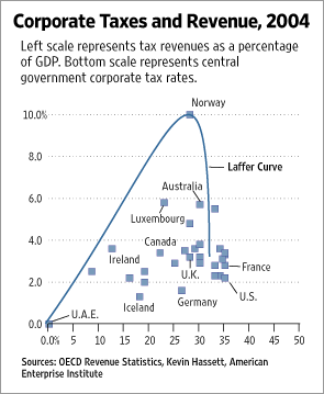
The data are in the rethinking package under the name Laffer. Fit two models to the data: one with a straight line and one with an actual curve. Compare these models using PSIS or WAIC. What do you conclude?
Click to see the answer
data(Laffer, package = "rethinking")
d <- Laffer
d <- d %>%
  mutate(across(everything(), rethinking::standardize))

m_straight = brm(
  data=d,
  family = gaussian,
  tax_revenue ~ tax_rate,
  prior = c( prior(normal(0,.1), class=Intercept),
             prior(normal(0,.5), class=b),
             prior(exponential(1), class=sigma)),
  iter=3000, warmup=1000, seed=9, chains=4,
  file = here("files/models/hw4.1")
)

m_curve = brm(
  data=d,
  family = gaussian,
  tax_revenue ~ tax_rate + I(tax_rate^2),
  prior = c( prior(normal(0,.1), class=Intercept),
             prior(normal(0,.5), class=b),
             prior(exponential(1), class=sigma)),
  iter=3000, warmup=1000, seed=9, chains=4,
  file = here("files/models/hw4.2")
)

m_straight <- add_criterion(m_straight, criterion = "loo")
m_straight <- add_criterion(m_straight, criterion = "waic")

m_curve <- add_criterion(m_curve, criterion = "loo")
m_curve <- add_criterion(m_curve, criterion = "waic")loo_compare(m_straight, m_curve, criterion = "loo") %>% print(simplify=F) elpd_diff se_diff elpd_loo se_elpd_loo p_loo se_p_loo looic se_looic
m_curve 0.0 0.0 -42.5 9.6 5.1 3.8 85.0 19.3
m_straight -0.8 0.9 -43.3 9.7 4.8 3.8 86.6 19.5 loo_compare(m_straight, m_curve, criterion = "waic") %>% print(simplify=F) elpd_diff se_diff elpd_waic se_elpd_waic p_waic se_p_waic waic
m_curve 0.0 0.0 -42.0 9.2 4.5 3.4 83.9
m_straight -1.0 0.9 -42.9 9.4 4.5 3.4 85.9
se_waic
m_curve 18.4
m_straight 18.8 - In the problem above, Norway is an outlier. Use PSIS or WAIC to estimate how much influence it has on the models you fit in the previous question.
Click to see the answer
Let’s start by identifying Norway. It has a very high tax revenue, so I’ll find the data point with the highest revenue.
(which_norway = which( d$tax_revenue == max(d$tax_revenue) ))[1] 12Point 12! Let’s see how it does on my statistics.
loo(m_straight)$pointwise[ which_norway, ] elpd_loo mcse_elpd_loo p_loo looic
-10.7496180 0.1598491 3.7979043 21.4992360
influence_pareto_k
0.9155318 loo(m_curve)$pointwise[ which_norway, ] elpd_loo mcse_elpd_loo p_loo looic
-10.6598434 0.2281193 3.8598310 21.3196868
influence_pareto_k
1.0607814 waic(m_straight)$pointwise[ which_norway, ] elpd_waic p_waic waic
-10.419245 3.467531 20.838489 waic(m_curve)$pointwise[ which_norway, ] elpd_waic p_waic waic
-10.182644 3.382631 20.365287 Very high influence on all of these lines. Let’s take just the first one: The influence according to PSIS on the straight curve is 0.92, which is a magnitude larger than almost all other influence metrics. It’s between .7 and 1, which puts it in the “bad” range (but not “very bad”), so take that for what it’s worth.